Learn how machines make decisions through experience instead of instructions.
Artificial Intelligence has evolved from a fascinating academic concept into one of the most transformative technologies of the modern world. Today, AI powers recommendation systems on Netflix and Spotify, assists doctors in diagnosing diseases, enables self-driving cars to navigate busy streets, optimizes warehouse robots, and even defeats world champions in complex strategy games.
But have you ever wondered how these systems actually learn what to do?
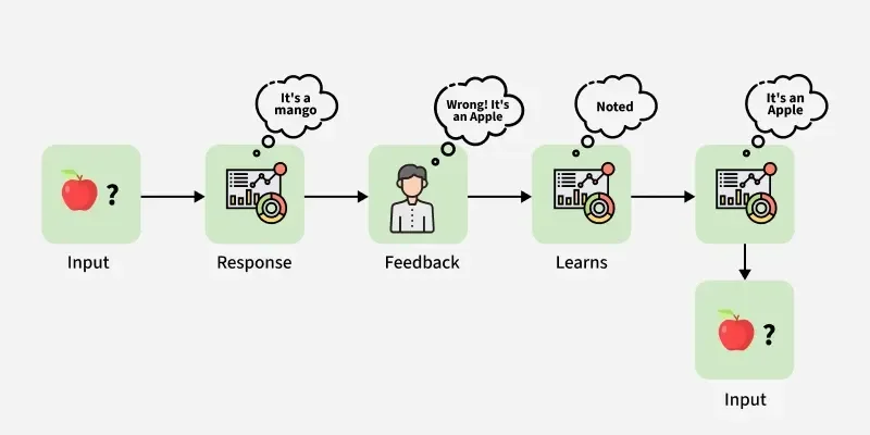
Unlike traditional software, where every rule must be explicitly programmed, many intelligent systems learn through experience. They make decisions, observe the outcomes, receive rewards or penalties, and gradually improve over time. This ability to learn from interaction is known as Reinforcement Learning, and one of its most influential algorithms is Q-Learning.
Introduced by Christopher Watkins in 1989, Q-Learning remains one of the most important algorithms in artificial intelligence. Although modern reinforcement learning has advanced significantly with deep neural networks and large-scale computing, the fundamental ideas behind today’s most successful reinforcement learning systems still originate from Q-Learning.
Whether you’re a computer science student, machine learning engineer, software developer, researcher, or simply curious about AI, understanding Q-Learning provides a strong conceptual foundation for learning more advanced algorithms such as Deep Q Networks (DQN), Proximal Policy Optimization (PPO), and Actor-Critic methods.
In this comprehensive guide, we’ll explore Q-Learning from first principles. Instead of simply memorizing equations, you’ll understand why the algorithm works, how it learns, where it’s used in the real world, and when it should—or shouldn’t—be applied.
What You’ll Learn
By the end of this guide, you’ll understand:
- What Q-Learning is and why it’s important
- The fundamentals of Reinforcement Learning
- How AI agents learn through trial and error
- The concepts of states, actions, rewards, and policies
- The intuition behind the Q-Learning algorithm
- The mathematical formula explained step by step
- Real-world applications in robotics, gaming, finance, healthcare, and autonomous systems
- Python implementation from scratch
- Advantages and limitations of Q-Learning
- How it compares with SARSA and Deep Q Networks (DQN)
- Common mistakes beginners make and best practices for implementing RL systems
TL;DR
If you’re looking for the short version, here’s what you need to know.
Q-Learning is a reinforcement learning algorithm that enables an intelligent agent to learn optimal decisions through experience rather than explicit programming.
Instead of relying on labeled datasets like supervised learning, the algorithm interacts with an environment, performs actions, receives rewards or penalties, and gradually learns which actions maximize long-term success.
Key facts:
- Model-free reinforcement learning algorithm that learns using trial and error
- Stores knowledge inside a Q-table to maximize future cumulative rewards
- Foundation of modern RL techniques used in robotics, games, and optimization
Why Should You Learn Q-Learning?
Many beginners rush directly into deep learning and large language models without understanding how intelligent decision-making actually works. Learning Q-Learning teaches you core concepts that appear throughout modern AI, including decision making, sequential planning, optimization, exploration, long-term reward maximization, and policy learning.
Even if you eventually work with sophisticated algorithms such as AlphaGo or autonomous vehicle systems, the underlying intuition often begins with Q-Learning. Think of it as learning algebra before calculus.
What Is Reinforcement Learning?
Machine learning is generally divided into three major categories: Supervised Learning (learning from labeled examples), Unsupervised Learning (finding hidden patterns), and Reinforcement Learning (learning through interaction).
| Learning Type | How It Learns | Example |
|---|---|---|
| Supervised Learning | Learns from labeled examples | Spam detection |
| Unsupervised Learning | Finds hidden patterns | Customer segmentation |
| Reinforcement Learning | Learns through interaction | Game-playing AI |
Reinforcement Learning (RL) differs from traditional machine learning because there are no correct answers provided during training. Instead, an intelligent agent must discover successful strategies by interacting with its environment.
Every decision leads to consequences: good decisions produce rewards, while poor decisions produce penalties. Over time, the agent learns how to maximize the total reward it receives. Imagine teaching a child to ride a bicycle: you don’t calculate the perfect balance equation for them; instead, they practice, fall, adjust, and improve until riding becomes second nature. Q-Learning follows a similar process.
Understanding the Reinforcement Learning Cycle
Every reinforcement learning problem follows the same basic interaction loop:
graph TD
    A[Environment] -->|Observe State & Reward| B[Agent]
    B -->|Select Action| A
The cycle repeats continuously:
- The agent observes its current state.
- It selects an action based on its current knowledge.
- The environment reacts, and the agent receives a reward signal.
- The environment transitions into a new state, and the process repeats.
Thousands—or even millions—of these interactions gradually produce intelligent behavior.
What Exactly Is Q-Learning?
Q-Learning is a model-free reinforcement learning algorithm that learns the value of taking a particular action in a particular state. Rather than memorizing entire paths or predefined rules, it estimates the quality of every possible decision.
The letter Q stands for Quality. Specifically, it answers: “How good is it to perform Action A while in State S?”
If the estimated value is high, the agent prefers that action. If the value is low, it avoids it. Eventually, every state develops a preferred action, and connecting all these preferred actions together creates an optimal strategy for solving the problem.
A Simple Real-World Analogy
Imagine you’ve just moved to a new city and need to drive to work every morning. Initially, you know nothing about the roads, so you experiment.
On Monday you try Route A and hit heavy traffic. On Tuesday you try Route B and encounter road construction. On Wednesday you try Route C and find a fast highway. By Thursday, you choose Route C again. After several weeks, you’ve learned which route consistently gets you to work fastest. Nobody explicitly taught you; you learned entirely from experience. That is essentially how Q-Learning works, except that instead of measuring travel time, an AI agent measures rewards.
The Four Building Blocks of Q-Learning
Every reinforcement learning problem consists of four essential components:
- Agent: The learner or decision maker (e.g., a robot, self-driving car, chess AI, or trading algorithm).
- Environment: Everything the agent interacts with (e.g., a warehouse, chessboard, road network, or video game).
- State: A snapshot of the current situation (e.g., robot standing at position (5,4)). The state answers: “Where am I right now?”
- Action: Every possible decision the agent can make (e.g., move left, accelerate, brake, or buy stock).
Reward Feedback
After every action, the environment provides feedback in the form of a reward. Positive rewards encourage behavior, while negative rewards discourage it.
| Action | Reward |
|---|---|
| Reach destination | +100 |
| Hit obstacle | -50 |
| Waste time | -2 |
| Collect treasure | +20 |
Over time, the agent discovers which sequence of actions produces the highest cumulative reward rather than simply chasing immediate gains.
How Does Q-Learning Work? The Learning Cycle
At its core, Q-Learning is surprisingly simple. An intelligent agent repeatedly interacts with an environment, makes decisions, receives feedback, and gradually learns which actions lead to the greatest long-term rewards.
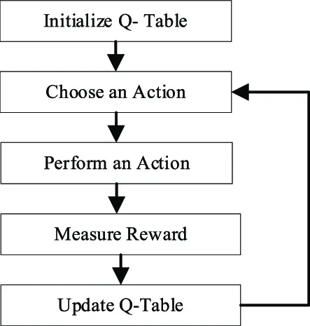 The fundamental Q-Learning interaction loop.
The learning cycle follows six precise steps:
- Observe State: The agent observes its current location and conditions in the environment.
- Select Action: The agent chooses an action using an exploration strategy.
- Interact: The environment processes the action and transitions to a new state.
- Receive Reward: The environment returns a numerical reward or penalty.
- Update Q-Value: The agent updates its Q-table using the Bellman equation.
- Repeat: The loop continues for thousands of episodes until the Q-values converge.
Understanding the Q-Learning Formula
The intelligence behind Q-Learning comes from a single update equation derived from the Bellman optimality equation:
Q(s,a) = Q(s,a) + α * [ R + γ * max_a' Q(s',a') - Q(s,a) ]This equation updates the estimated quality of taking action a while in state s. Instead of replacing previous knowledge entirely, the algorithm slightly adjusts it after every experience using the learning rate $\alpha$.
Formula Breakdown
- $Q(s,a)$: The current estimate of taking action $a$ in state $s$.
- Learning Rate ($\alpha$): Controls how quickly new information overwrites old knowledge (typically 0.1 to 0.5).
- Reward ($R$): The immediate reward returned by the environment.
- Discount Factor ($\gamma$): Determines how much future rewards matter relative to immediate rewards (typically 0.90 to 0.99).
- $\max_{a’} Q(s’,a’)$: The estimated maximum future reward achievable from the next state $s’$.
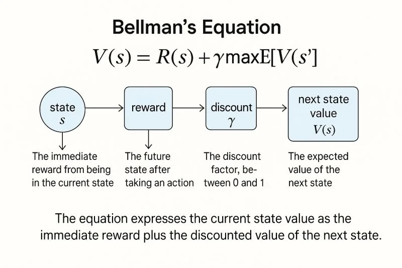 Visualization of the Bellman equation and temporal difference update.
What Is a Q-Table?
The Q-table is the agent’s memory. Every row represents a state, every column represents an action, and each cell stores the estimated cumulative future reward.
| State | Left | Right | Up | Down |
|---|---|---|---|---|
| State A | 12.4 | 45.1 | 8.0 | 21.3 |
| State B | 18.2 | 73.8 | 40.0 | 7.1 |
| State C | 5.0 | 22.4 | 81.6 | 14.2 |
| State D | 64.9 | 18.0 | 13.5 | 9.0 |
Initially, every cell in the table is initialized to zero or small random values. As training progresses, the numbers become increasingly accurate until the highest value in each row represents the optimal decision.
Exploration vs. Exploitation ($\epsilon$-Greedy)
One of the biggest challenges in reinforcement learning is balancing curiosity with confidence:
- Exploration: Trying new actions to discover potentially better strategies.
- Exploitation: Using the best-known action to maximize current reward.
The standard solution is the $\epsilon$-greedy policy. With probability $\epsilon$, the agent picks a random action to explore; with probability $1-\epsilon$, it selects the action with the highest Q-value. Typically, $\epsilon$ starts at 1.0 (pure exploration) and gradually decays over training to 0.05 (pure exploitation).
Interactive Grid World & Parameter Simulator
Test Q-Learning live in your browser! Adjust $\alpha$, $\gamma$, and $\epsilon$ to watch how the Q-table updates in real-time.
Implementing Q-Learning in Python
Below is a complete, clean Python implementation of a Q-Learning training loop using NumPy:
import numpy as np

# Initialize environment dimensions and parameters
num_states = 16
num_actions = 4

Q = np.zeros((num_states, num_actions))

alpha = 0.1    # Learning rate
gamma = 0.95   # Discount factor
epsilon = 0.2  # Exploration rate

# Simplified training loop
for episode in range(1000):
    state = 0  # Start state
    done = False

    while not done:
        # Epsilon-greedy action selection
        if np.random.random() < epsilon:
            action = np.random.randint(0, num_actions)
        else:
            action = np.argmax(Q[state])

        # Execute action in environment (simulated step)
        next_state = (state + 1) % num_states
        reward = 100 if next_state == 15 else -1
        done = (next_state == 15)

        # Q-Learning update rule (Bellman equation)
        best_next_q = np.max(Q[next_state])
        Q[state, action] += alpha * (reward + gamma * best_next_q - Q[state, action])

        state = next_state
💡 Did You Know?
The simple code above captures the core learning mechanism of modern AI. Advanced algorithms replace the 2D NumPy array with deep neural networks, but the Bellman temporal difference logic remains identical.
Q-Learning vs. SARSA vs. Deep Q Networks (DQN)
As reinforcement learning evolved, several algorithms were developed to overcome the scaling limitations of traditional Q-Learning.
| Feature | Q-Learning | SARSA | Deep Q Network (DQN) |
|---|---|---|---|
| Policy Type | Off-Policy | On-Policy | Off-Policy |
| State Memory | Q-Table | Q-Table | Neural Network |
| Next Action Target | $\max_{a’} Q(s’, a’)$ | $Q(s’, a_{actual}’)$ | Neural Net $\max_{a’} Q(s’, a’)$ |
| Best Used For | Small discrete grid worlds | Safe physical robotics | High-dimensional inputs (Pixels/Atari) |
| Training Speed | Fast convergence | Conservative / Stable | Requires GPU acceleration |
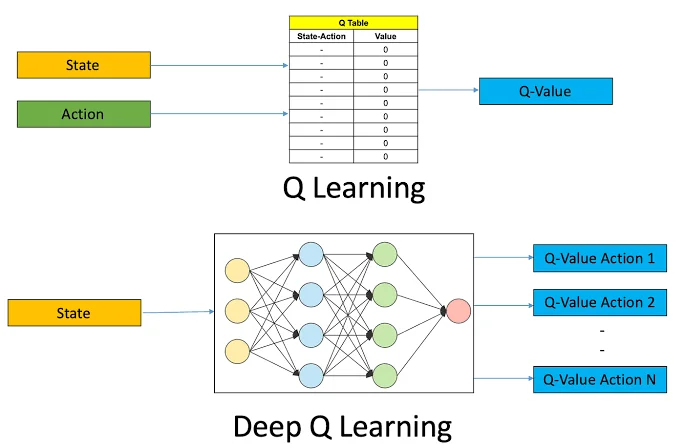 Deep Q Networks replace the tabular memory with deep neural network function approximation.
Real-World Applications
While Q-Learning is often demonstrated in grid worlds, its underlying principles power major industrial systems:
- Robotics & Automation: Warehouse inventory routing, robotic arm manipulation, and drone navigation.
- Autonomous Vehicles: Strategic decision making for lane changes, speed adaptation, and traffic flow optimization.
- Recommendation Engines: Personalizing content recommendations on platforms like Netflix and YouTube to maximize long-term engagement.
- Finance & Algorithmic Trading: Portfolio rebalancing, automated risk management, and dynamic asset allocation.
- Healthcare: Optimizing personalized treatment plans and dynamic medical resource scheduling.
Common Mistakes Beginners Make
Avoid these common pitfalls when building your first reinforcement learning model:
- Setting $\alpha$ too high: A learning rate of 1.0 causes Q-values to oscillate wildy without converging. Keep $\alpha$ between 0.05 and 0.2.
- Premature Epsilon Decay: Decaying $\epsilon$ to zero too quickly freezes exploration before the optimal path is discovered.
- Flawed Reward Design: Giving positive rewards for intermediate moves can cause agents to run in circles endlessly to farm points.
- Expecting Instant Convergence: Reinforcement learning is an iterative optimization process that requires hundreds or thousands of episodes.
Frequently Asked Questions
Is Q-Learning still relevant in 2026?
Yes! While Deep RL algorithms like PPO and SAC handle high-dimensional continuous control, Q-Learning remains the essential foundational algorithm for understanding reinforcement learning theory, Q-tables, and temporal difference updates.
Why is Q-Learning called “model-free”?
Because it does not require a mathematical model of the environment’s transition probabilities. The agent learns optimal actions purely through direct interaction and trial-and-error experience.
What is the difference between Q-Learning and Deep Q-Learning (DQN)?
Q-Learning uses a 2D lookup table (Q-table) to store values for discrete states. Deep Q-Learning replaces the table with a deep neural network, enabling the algorithm to handle complex continuous inputs like video pixels.
How do I choose between Q-Learning and SARSA?
Use Q-Learning when you want to learn the absolute optimal policy aggressively from replay data. Use SARSA when training in physical environments where taking risky exploratory actions could cause hardware damage.